2.4. Hyperparameter Optimization#
In Section 2.3, we mention the concepts of model parameters and hyperparameters. Hyperparameters refer to parameters that lie outside the model parameters, such as the learning rate that controls the speed of gradient descent during the training of deep learning models, or the number of branches in a decision tree. Hyperparameters typically fall into two categories:
Model: The design of the neural network, such as the number of layers, the size of the convolutional kernels, and the number of branches in a decision tree.
Training and Algorithms: Learning rate, batch size, etc.
Search Algorithms#
The method of determining these hyperparameters involves initiating multiple trials, where each trial tests a specific value of the hyperparameters. Selection is made based on the quality of the model training results. This process is known as hyperparameter tuning. The search for optimal hyperparameters can be conducted manually, but this is time-consuming and inefficient, leading to the academia and industry proposing some automated methods. Common automated search methods are as follows, and Fig. 2.6 illustrates hyperparameter search in a two-dimensional search space, where each point represents a combination of hyperparameters, with warmer colors indicating better performance. Iterative algorithms start from an initial point and subsequent trials depend on the results of previous trials, eventually converging towards the direction of better performance.

Fig. 2.6 In a two-dimensional search space, hyperparameter tuning is conducted where each point represents a combination of hyperparameters, with warmer colors indicating better performance and cooler colors indicating worse performance.#
Grid Search: Grid search is an exhaustive search method that seeks the optimal solution by traversing all possible combinations of hyperparameters. These combinations are used one by one to train and evaluate the model. Grid search is simple and intuitive, but when the hyperparameter space is large, the computational cost increases dramatically.
Random Search: Random search does not traverse all possible combinations but instead randomly selects combinations of hyperparameters for evaluation within the solution space. This method is usually more efficient than grid search because it does not require evaluating all possible combinations, but explores the parameter space through random sampling. Random search is particularly suitable for situations where the hyperparameter space is very large or has high dimensionality, as it can find a good hyperparameter configuration in fewer attempts. However, due to its randomness, random search may miss some local optimal solutions, thus requiring more attempts to ensure a good solution is found.
Adaptive Selection: The most well-known technique in adaptive hyperparameter search is Bayesian Optimization. Bayesian optimization is based on Bayesian theorem and probabilistic models to guide the search for optimal hyperparameters. The core idea of this method is to construct a Bayesian model, typically a Gaussian Process, to approximate the unknown part of the objective function. Bayesian optimization can intelligently select the most promising hyperparameter combinations within a limited number of evaluations, especially suitable for scenarios with high computational costs.
Hyperparameter tuning is a kind of black-box optimization, where the term black-box optimization refers to the objective function being a black box; we can only infer its behavior by observing its inputs and outputs. The concept of a black box is relatively difficult to understand, but we can compare it with gradient descent algorithms, which are not black-box optimization algorithms. We can obtain the gradient (or the approximation of the gradient) of the objective function and use the gradient to guide the search direction, ultimately finding the (local) optimal solution of the objective function. Black-box optimization algorithms generally cannot find the mathematical expression and gradient of the objective function, nor can they use gradient-based optimization techniques. Bayesian optimization, genetic algorithms, simulated annealing, etc., are all black-box optimizations. These algorithms typically select some candidate solutions in the hyperparameter search space, run the objective function, obtain the actual performance of the hyperparameter combination, and based on the actual performance, continuously iterate and adjust, that is, repeat the above process until conditions are met.
Bayesian Optimization#
Bayesian optimization is based on the Bayesian theorem, and we will not delve into the detailed mathematical formulas here. Simply put, it requires initially grasping the actual performance of a few observed sample points in the search space, building a probabilistic model that describes the mean and variance of the model performance metric at each value of every hyperparameter. The mean represents the expected effect of this point, where a larger mean indicates a better model performance metric, and the variance indicates the uncertainty of this point; a larger variance suggests greater uncertainty and is worth exploring. Fig. 2.7 illustrates the iterative process of 3 iterations in a 1-dimensional hyperparameter search space, where the dashed line is the true value of the Objective Function, the solid line is the predicted value (or posterior probability distribution mean), and the blue area above and below the solid line represents the confidence interval. Bayesian optimization utilizes a Gaussian Process, meaning the objective function is a stochastic process composed of a series of observations, described by a Gaussian probabilistic model. Bayesian optimization continuously updates the posterior distribution of the objective function by collecting observations until the posterior distribution closely fits the true distribution. In the case of Fig. 2.7, before the 3rd iteration, there were only two observations, and after the 3rd and 4th iterations, new observed sample points were added, with the predicted values near these points gradually approaching the true values.
Bayesian optimization has two core concepts:
Surrogate Model: The surrogate model fits the observed values and predicts actual performance, which can be understood as the solid line in the graph.
Acquisition Function: The acquisition function is used to select the next sampling point. It uses some methods to measure the contribution of each point to the optimization of the objective function, which can be understood as the orange line in the graph.
To prevent falling into a local optimum, the acquisition function should consider both Exploiting those with larger means and Exploring those with larger variances when selecting the next value point. That is, finding a balance between Exploit and Explore. For example, if model training is very time-consuming and limited computational resources can only run 1 set of hyperparameters, one should choose the one with the larger mean, as this has the highest possibility of selecting the optimal result; if our computational resources can run thousands of times, then we should explore different possibilities. In the example of Fig. 2.7, the 3rd iteration and the 2nd iteration both select new points near the observed value of the 2nd iteration, which is a balance between exploration and exploitation.

Fig. 2.7 How to choose the next point after several iterations of Bayesian optimization.#
Compared to grid search and random search, Bayesian optimization is not easily parallelizable because it requires running some hyperparameter combinations first to obtain some actual observed data.
Scheduler#
Successive Halving Algorithm#
The core idea of the Successive Halving Algorithm (SHA) [Karnin et al., 2013] is quite straightforward as depicted in Fig. 2.8:
Initially, SHA allocates a certain amount of computational resources to each hyperparameter combination.
After training and executing these hyperparameter combinations, the results are evaluated.
The hyperparameter combinations that rank higher are selected for the next round (Rung) of training, while those with poor performance are stopped early.
In the next rung, the computational resource quota for each hyperparameter combination is increased according to a certain strategy.

Fig. 2.8 Optimizing the minimum of a metric using SHA algorithm.#
The computational resource budget, also known as the “Budget,” can be the number of training iterations or the amount of training data, among other metrics. More precisely, in each rung of the SHA algorithm, a fraction of the hyperparameter combinations is discarded, specifically \( \frac{\eta - 1}{\eta} \), while \( \frac{1}{\eta} \) of the combinations are passed to the next rung. In the subsequent rung, the computational resource quota for each hyperparameter combination is increased to \( \eta \) times its original amount.
In the context of Table 2.1, the total computational resources available per rung are denoted by \( B \), with a total of 81 hyperparameter combinations under consideration. In the first rung, each trial is allocated a fraction of the total resources, which is \( \frac{B}{81} \). Assuming \( \eta \) is set to 3, only \( \frac{1}{3} \) of the trials, based on their performance, will be promoted to the next round. After five rounds of this process, the optimal hyperparameter combination will be selected.
Number of Hyperparameters \(n\) |
Budget of each trail \(\frac{B}{n}\) |
|
|---|---|---|
Rung 1 |
81 |
\(\frac{B}{81}\) |
Rung 2 |
27 |
\(\frac{B}{27}\) |
Rung 3 |
9 |
\(\frac{B}{9}\) |
Rung 4 |
3 |
\(\frac{B}{3}\) |
Rung 5 |
1 |
\(B\) |
In the SHA, it is necessary to wait for all hyperparameter combinations in the same rung to complete training and have their results evaluated before proceeding to the next rung. Initially, multiple trials can be executed in parallel during the first round. However, as the process advances to subsequent rounds, the number of trials decreases, leading to lower parallelism. The Asynchronous Successive Halving Algorithm (ASHA) is an optimization of SHA. ASHA does not require waiting for the completion of training and evaluation of a rung to select candidates for the next rung. Instead, it allows for the selection of hyperparameter combinations that can be promoted to the next round while the current round is still in progress. This means that the training and evaluation of the previous round and the next rung are carried out concurrently.
The main assumption in both the SHA and the ASHA algorithm is that if a trial performs well initially, it will continue to perform well in future rounds. This assumption is, of course, overly simplistic. A counterexample is the learning rate: a higher learning rate may perform better than a lower one in the short term, but it may not be optimal in the long run. The SHA scheduler could mistakenly terminate trials with lower learning rates early. From another perspective, to avoid the early termination of potentially promising trials, it would be beneficial to allocate more computational resources to each trial in the first round. However, due to the limited total computational budget \( B \), a compromise is to select fewer hyperparameter combinations, meaning the number of combinations, denoted as \( n \), should be smaller.
Hyperband#
Algorithms such as SHA and ASHA face the challenge of balancing between \(n\) and \(\frac{B}{n}\): if \(n\) is too large, each trial may have insufficient resources, leading to the early termination of promising trials; if \(n\) is too small, the search space is limited, which may also result in the exclusion of potentially high-performing trials from the search. The HyperBand algorithm introduces a hedging mechanism based on SHA. HyperBand is somewhat akin to a financial investment portfolio, using a variety of financial assets to hedge against risks. The initial round is not a fixed \(n\) but has multiple possible \(n\) values. As shown in Fig. 2.9, in terms of implementation, HyperBand uses two nested loops, with the inner loop directly invoking the SHA algorithm, and the outer loop trying different \(n\) values, each possibility being a \(s\). HyperBand additionally introduces the variable \(R\), which refers to the maximum computational resource budget for a hyperparameter combination, and \(s_{max}\) is the total number of possibilities, which can be calculated as: \(\lfloor \log_{\eta}{R} \rfloor\); due to the introduction of \(R\), the total computational resource \(B\) is now \((s_{max} + 1)R\), with the addition of one because \(s\) is calculated starting from 0.
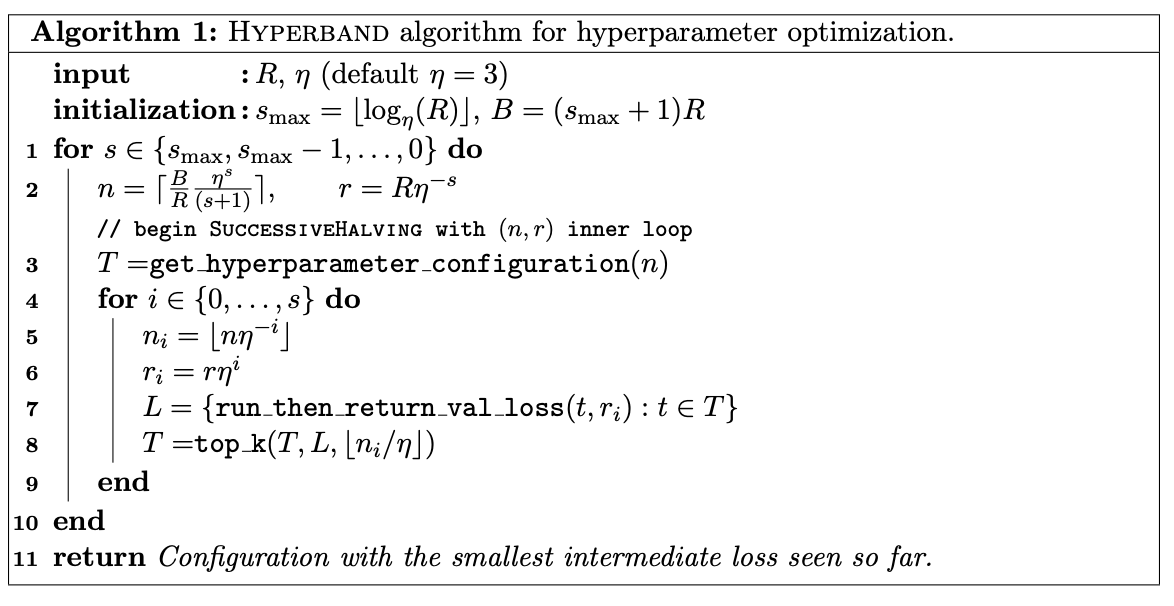
Fig. 2.9 The HyperBand Algorithm#
Fig. 2.10 is an illustrative example: the horizontal axis represents the outer loop, which has 5 possibilities (ranging from 0 to 4), and the initial computational resources \(n\) along with the computational resources \(r\) that each hyperparameter combination can obtain form a Bracket; the vertical axis represents the inner loop, where for a given initial Bracket, the SHA algorithm is executed, iterating until the optimal trial is selected.

Fig. 2.10 Illustration of the Hyperband algorithm.#
BOHB#
BOHB [Falkner et al., 2018] is a scheduler that combines the strengths of both Bayesian Optimization and Hyperband.
Population Based Training#
Population Based Training (PBT) [Jaderberg et al., 2017] is primarily aimed at the training of deep neural networks, drawing inspirations from genetic algorithms to simultaneously optimize model parameters and hyperparameters. In PBT, the population can be simply understood as different trials. PBT launches multiple trials in parallel, each trial randomly selects a combination of hyperparameters from the search space and initializes the model parameter, and the model metrics are regularly assessed during the training process. During the model training process, based on the model performance metrics, PBT will either exploit or explore the model parameters or hyperparameters of the current trial. If the current trial’s metrics are not satisfactory, PBT will exploit model weights of those better-performing models. PBT explores by generating new hyperparameters for subsequent training. Throughout a complete training process, other hyperparameter tuning methods can only select hyperparameters; PBT, however, can optimize both model parameters and hyperparameters simultaneously.

Fig. 2.11 Exploit and explore in PBT. Exploit refers to using model weights from other better-performing weights, while explore means using new hyperparameter combination through mutation.#